From Lines to Layers: The Linear Perceptron and the Rise of Neural Networks
At the heart of today's neural networks lies a surprisingly simple idea: the perceptron. How it works, how it learns to separate data, and how stacking these units leads to powerful models.
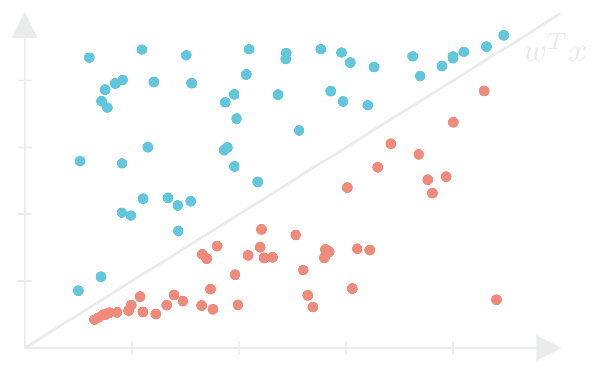
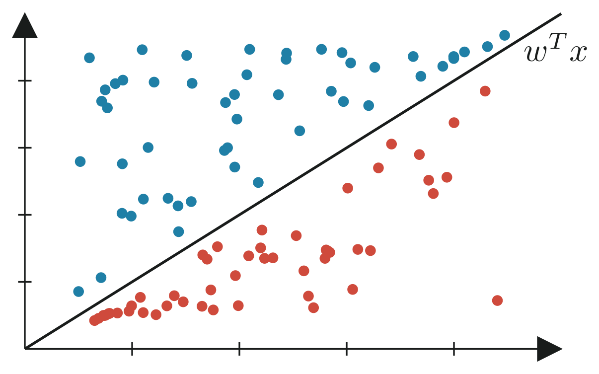
At its core, the linear perceptron is like a tiny decision maker. It takes a set of inputs, weighs how important each input is, and produces one of two outputs: yes or no, 1 or 0, apples or oranges. Imagine a straight line cutting through a 2D space: everything on one side is classified as one thing, everything on the other side is classified as something else. Each example we test becomes a data point in that space, and the perceptron decides which side of the line it belongs on.
The linear perceptron is a supervised learning algorithm that is a binary classifier—meaning it tries to separate data into two categories. It learns by comparing its predictions with the expected answers and adjusting its weights until it draws a line that correctly divides the two classes.
A Sweet Example
Let’s say we want to predict whether a user will click on an ad for ice cream. Naturally, most people don’t click on ads, so we shift our decision boundary a bit to account for this tendency. This shift is called the bias. We also have other information about the user:
-
Searched for “ice cream”
-
Recently bought ice cream
-
Is lactose intolerant
We can put this information about our user into a feature vector and assign a weight to each input. To include the bias, we add an extra feature with a constant value of 1 and give it its own weight :
We then take the dot product of these two vectors. This gives us a single number that represents the combined influence of all the points. To turn that number into a decision (click or no click) we pass it through an activation function:
Activation Functions
An activation function is like a switch:
-
If the total score is high enough, the switch turns on (click)
-
If its too low, the switch stays off (no click)
For a simple linear perceptron, this “switch” is a step function:
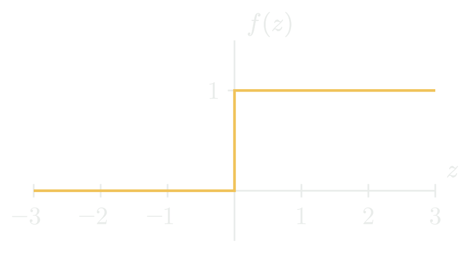
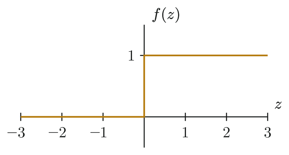
Where the score, , is our weighted sum of inputs. Without an activation function, our perceptron would just spit out numbers. The activation function is what turns those numbers into decisions.
What happens when ?
By convention, ties that lie exactly on the decision boundary go the positive class.
Learning the Weights
1. Start With a Guess
We begin by assigning random weights to each input. At first, the perceptron is just guessing where the boundary should be and will produce subpar predictions.
2. Make Predictions
For each data point, we calculated the predicted output (either 0 or 1):
3. Compare
Because the linear perceptron is a supervised learning algorithm, we know the correct output. If the prediction was wrong, we need to adjust the weights.
4. Adjusting the Weights
For each incorrectly classified data point, we nudge its weights to make better predictions next time. The update rule looks like this:
Where:
- is the correct output
- is the predicted output
- is the weight vector we are updating
- is the learning rate, or how much we should adjust the weights
- is the training iteration
This is essentially saying:
- If the perceptron guessed too low when the answer was yes: increase weights for those inputs.
- If the perceptron guessed too high when the answer was no: decrease weights.
5. Repeat
Repeat steps 2-4 many times until the model either correctly predicts each data point, or we have exceeded the maximum number of iterations. We will see later why we need to set a limit on the number of training iterations.
Back to Our Ice Cream Example
Let’s walk through an iteration of our training algorithm and see how the model adjusts its weights to make better predictions.
- Inputs: (bias = 1, searched “ice cream”, not lactose intolerant)
- Current Weights:
- Correct Output: (they clicked)
- Initial Prediction: (perceptron says no)
- Learning Rate:
Update Step:
Comparing Predictions
Before the weight update:
The model guessed wrong. After the update:
The perceptron now predicts correctly. This is learning in action, the model shifts its decision boundary a little closer to the right answer after each mistake.
Limitations of a Single Perceptron
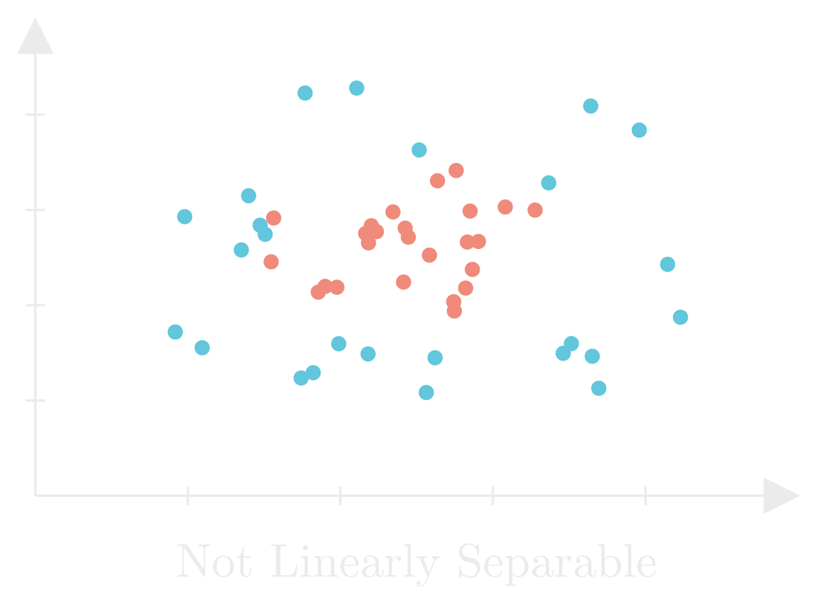
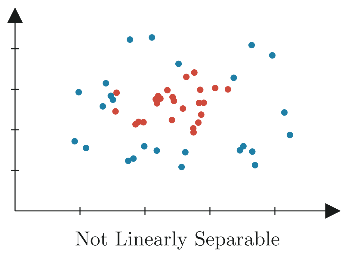
Our example shows a case where the data can be separated by a straight line, the perceptron just had to learn where to put it. But what if the data can’t be split cleanly by any line at all?
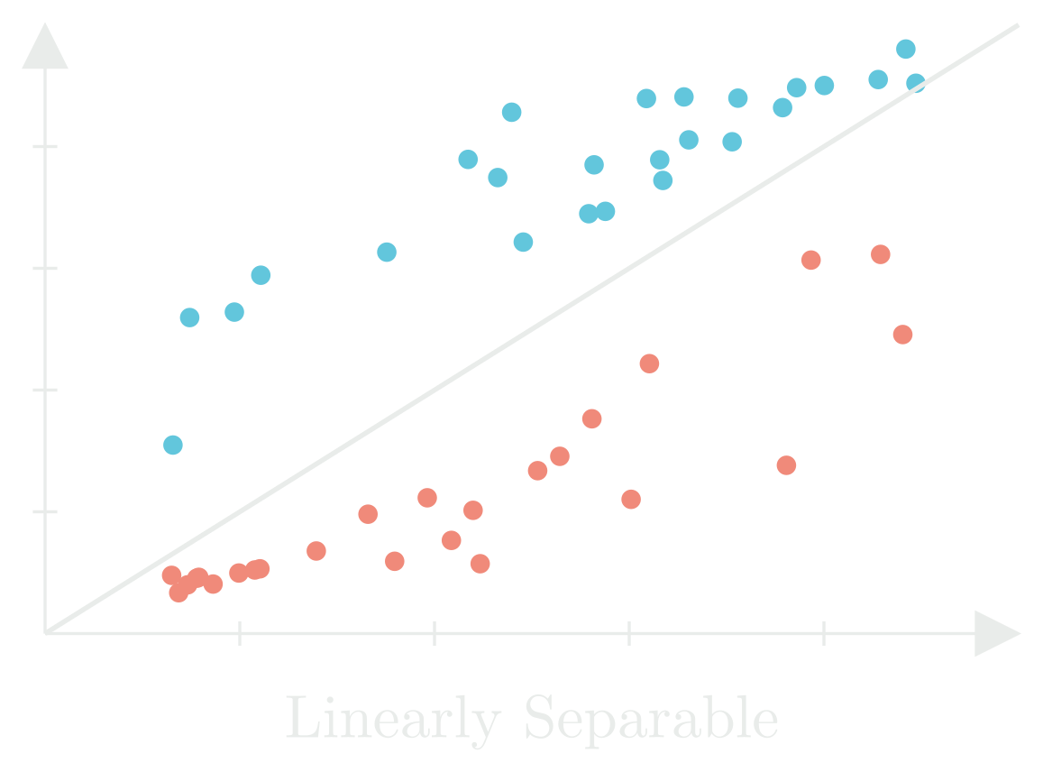
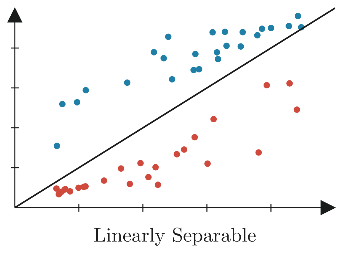
If the data points are linearly separable, our perceptron algorithm is guaranteed by the Perceptron Convergence Theorem to find a set of weights that correctly classifies every point in a finite number of steps.
If the data points are not linearly separable, no straight-line classifier can perfectly separate them. In this case, the perceptron will continue adjusting its weights indefinitely, oscillating between solutions without ever reaching a perfect classification. That’s why we usually set a limit on the number of iterations or another stopping condition to prevent infinite training.
The XOR Problem
The XOR (exclusive OR) is a logical operation that results in true if and only if one of its inputs is true and the other is false. We can represent this behavior as both a truth table and a set of points on a 2D plane.
| XOR | ||
|---|---|---|
| 1 | 1 | 0 |
| 1 | 0 | 1 |
| 0 | 1 | 1 |
| 0 | 0 | 0 |
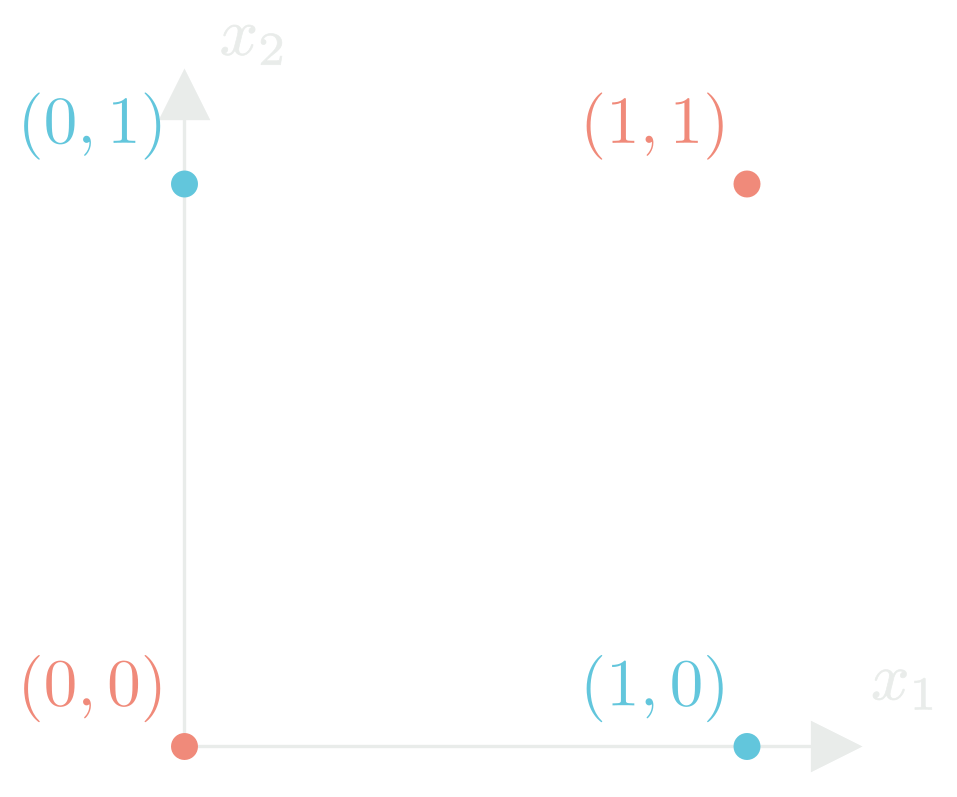
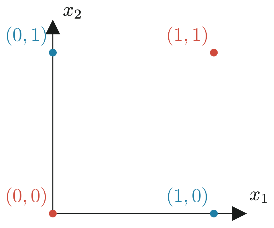
You can clearly see no matter how you draw a single straight line, you can’t perfectly separate the two classes. Points in opposite corners belong to the same class, meaning you’d need at least two lines or a curved boundary to classify them correctly.
This is the XOR Problem, a classic example that shows the limitations of a single perceptron.
Why This Was a Big Deal
Back in the 1960s, this wasn’t just a small inconvenience, it was a fundamental limitation of machine learning. After all, if we couldn’t teach a model to separate four points on a plane—how could we expect it to solve complex real-world problems? This discovery led to the first AI winter, a period where funding and interest in AI dropped sharply.
The Solution: More Neurons
Instead of just relying on one perceptron, you can stack many perceptrons into layers.
- The first layer can learn simple, straight-line boundaries
- The next layer can combine those boundaries to make more complex shapes
- Add non-linear activation functions (like sigmoid, ReLU, tanh), and suddenly networks can model curved, multi-step decision boundaries that a single perceptron never could.
This is the foundation of neural networks
From Perceptrons to Neural Networks
Each perceptron becomes an individual node inside a larger network. On its own, it draws one line. But together, in layers, these nodes can learn highly flexible decision boundaries.
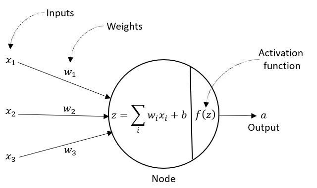
Over time, researchers improved training techniques (with enhancements like backpropagation) and computers got faster, enabling deep learning—networks with many layers and thousands or millions of nodes. These systems power everything from autonomous vehicles to large language models, but at their core, they’re still built on the same fundamental principle Rosenblatt introduced back in 1958:
Stack enough of these simple decision-makers together, and you can model just about anything.